Monday, June 30, 2014

Band offsets of lattice-matched semiconductor heterojunctions through hybrid functionals and G0W0

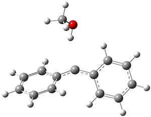
Karim Steiner, Wei Chen, and Alfredo Pasquarello Phys. Rev. B 89, 205309 
Contributed by David Bowler
Reposted from Atomistic Computer Simulations with permission

Fixing the well-known problems with DFT band gaps can be done, but there is no universal solution.  Hybrid functionals have long been used in the chemistry community (where B3LYP is very popular) while solid state approaches tend to use the PBE0 functional (which mixes 25% exact exchange into the PBE functional in its original form).  There are also many-body perturbation theory approaches such as GW, which tend to be complex but are generally very good at getting band structures correct.
The paper I’m writing about[1] considers how to calculate offsets between both the valence and conduction bands in different bulk semiconductors.  These have obvious applications in areas such as photovoltaics and electronics, and a consistent way to calculate them would be very valuable.  This isn’t the only paper which has been written about this problem; however, this paper is really very careful, and goes to some lengths to be open.  They give details of all the relevant parameters used in the calculations, even giving details of the pseudopotentials used.  This is unusual, and highly laudable: it makes the science they do open and reproducible.
They consider non-polar interfaces, and a range of group IV, III-V and II-VI semiconductors.  What do they find ? They use the common one-shot G0W0 method (which calculates corrections to DFT bands without any form of self-consistency) and find excellent agreement with experiment.  For PBE0, the hybrid functional, they find that the original mixing parameter of 0.25 gives poor results; they optimise it by fitting either to experimental gaps or to GW gaps.  When modelling the interfaces, they find that the experimental gap fitting process (taking an average of the values for the two semiconductors) is much better.  Interestingly, they find that the valence band offsets are modelled extremely well by PBE alone, though they have applied a similar method to semiconductor/insulator interfaces where PBE fared rather poorly[2].
Overall, the conclusions add to our understanding of hybrids and GW.  A single hybrid mixing parameter for all systems performs fairly poorly; however, fitting the parameter to (say) bulk properties can be successful.  GW is generally reliable, though it cannot calculate electron-hole effects, and can depend on input bands (in particular, small gap systems in DFT can form a poor starting point for GW calculations – see, for instance [3]).  But I really like their approach, constructing pseudopotentials very carefully and publishing their protocols.
[1] Phys. Rev. B 89, 205309 (2014) doi:10.1103/PhysRevB.89.205309
[2] Phys. Rev. Lett. 101, 106802 doi:10.1103/PhysRevLett.101.106802
[3] New J. Phys. 7 126 (2005) doi:10.1088/1367-2630/7/1/126

Wednesday, June 25, 2014

Total synthesis and isolation of citrinalin and cyclopiamine congeners

Mercado-Marin, E. V.; Garcia-Reynaga, P.; Romminger, S.; Pimenta, E. F.; Romney, D. K.; Lodewyk, M. W.; Williams, D. E.; Andersen, R. J.; Miller, S. J.; Tantillo, D. J.; Berlinck, R. G. S.; Sarpong, R. Nature 2014, 509, 318-324
Contributed by Steven Bachrach.
Reposted from Computational Organic Chemistry with permission

Here is another nice example of the partnership between experiment and computation in ascertaining molecular structure. The Sarpong, Tantillo and Miller groups collaborated on the synthesis, characterization and biosynthesis of some metabolites from Penniculium strains.1 I will focus here on just the structural identification component of this paper; the synthesis and the biosynthesis are very interesting too!

Cyclopiamine A 1 and cyclopiamine B 2 interconvert through an intermediate that allows for the epimerization at carbon bearing the nitro group.2

1

2
Citrinalin A 3 might also seem to undergo the same type of ring opening-ring closing reaction to produce citrinalin B. However, the original proposed structure3 of citrinalin B 4 implies an epimerization at a different carbon (at the ring fusion to the terminal 5 member ring). These authors suggested that perhaps the proper structure of citrinalin B is 5, which differs from citrinalin A only at the carbon bearing the nitro group, analogous to the relationship between 1 and 2.

3

4

5
The low energy conformations of both 4 and 5 (actually the trifluoroacetic acid salts) were optimized at B3LYP/6-31+G(d,p) and the chemical shifts for both 1H and 13C were computed, Boltzmann-weighted and scaled, and then compared with the NMR spectra of authentic citrinalin B. (The lowest energy conformations of 4 and 5 are shown in Figure 1.) The corrected mean absolute deviations for the 1H and13C chemical shift for the original structure 4 are 0.45 ppm and 2.0 ppm, respectively (with the largest outliers of 2.3 ppm for H and 9.6 ppm for C). These errors are about twice what is observed in comparing the experimental and computed 1H and 13C chemical shifts of 3. The agreement between the computed and experimental values using 5 are much improved, with mean deviations of 0.12 and 1.6ppm, and largest deviations of 0.38 ppm for 1H and 4.4 ppm for 13C. Use of Goodman’s DP4 method indicates a 100% probability that the structure of citrinalin B is 5. This prediction is confirmed by the x-ray structure.

4

5
Figure 1. B3LYP/6-31+G(d,p) optimized lowest energy conformers of 4 and 5.


References

(1) Mercado-Marin, E. V.; Garcia-Reynaga, P.; Romminger, S.; Pimenta, E. F.; Romney, D. K.; Lodewyk, M. W.; Williams, D. E.; Andersen, R. J.; Miller, S. J.; Tantillo, D. J.; Berlinck, R. G. S.; Sarpong, R. "Total synthesis and isolation of citrinalin and cyclopiamine congeners," Nature 2014509, 318-324, DOI:10.1038/nature13273.
(2) Bond, R. F.; Boeyens, J. C. A.; Holzapfel, C. W.; Steyn, P. S. "Cyclopiamines A and B, novel oxindole metabolites of Penicillium cyclopium westling," J. Chem. Soc., Perkin Trans I 1979, 1751-1761, DOI:10.1039/P19790001751.
(3) Pimenta, E. F.; Vita-Marques, A. M.; Tininis, A.; Seleghim, M. H. R.; Sette, L. D.; Veloso, K.; Ferreira, A. G.; Williams, D. E.; Patrick, B. O.; Dalisay, D. S.; Andersen, R. J.; Berlinck, R. G. S. "Use of Experimental Design for the Optimization of the Production of New Secondary Metabolites by Two Penicillium Species,"J. Nat. Prod. 201073, 1821-1832, DOI: 10.1021/np100470h.


InChIs

1: InChI=1S/C26H33N3O5/c1-23(2)12-17(30)20-18(34-5)9-8-16-21(20)28(23)22(31)26(16)13-25(29(32)33)14-27-10-6-7-15(27)11-19(25)24(26,3)4/h8-9,15,19H,6-7,10-14H2,1-5H3/t15-,19+,25+,26-/m1/s1
InChIKey=LUESCPPTDJZZQN-VBPSCBQFSA-N
2: InChI=1S/C26H33N3O5/c1-23(2)12-17(30)20-18(34-5)9-8-16-21(20)28(23)22(31)26(16)13-25(29(32)33)14-27-10-6-7-15(27)11-19(25)24(26,3)4/h8-9,15,19H,6-7,10-14H2,1-5H3/t15-,19+,25-,26-/m1/s1
InChIKey=LUESCPPTDJZZQN-DCWDXPITSA-N
3: InChI=1S/C25H31N3O5/c1-22(2)11-16(29)19-17(33-22)8-7-15-20(19)26-21(30)25(15)12-24(28(31)32)13-27-9-5-6-14(27)10-18(24)23(25,3)4/h7-8,14,18H,5-6,9-13H2,1-4H3,(H,26,30)/t14-,18+,24+,25-/m0/s1
InChIKey=QVBARITWSQCBBV-DTKOROOESA-N
4: InChI=1S/C25H31N3O5/c1-22(2)11-16(29)19-17(33-22)8-7-15-20(19)26-21(30)25(15)12-24(28(31)32)13-27-9-5-6-14(27)10-18(24)23(25,3)4/h7-8,14,18H,5-6,9-13H2,1-4H3,(H,26,30)/t14-,18-,24-,25+/m1/s1
InChIKey=QVBARITWSQCBBV-KUCRYEJDSA-N
5: InChI=1S/C25H31N3O5/c1-22(2)11-16(29)19-17(33-22)8-7-15-20(19)26-21(30)25(15)12-24(28(31)32)13-27-9-5-6-14(27)10-18(24)23(25,3)4/h7-8,14,18H,5-6,9-13H2,1-4H3,(H,26,30)/t14-,18+,24-,25-/m0/s1
InChIKey=QVBARITWSQCBBV-QBDGMKJCSA-N

This work is licensed under a Creative Commons Attribution-NoDerivs 3.0 Unported License.

Monday, June 23, 2014

Hydrogen Bonding Switches the Spin State of Diphenylcarbene from Triplet to Singlet

Costa, P.; Sander, W. Angew. Chem. Int. Ed. 2014, 53, 5122-5125
Contributed by Steven Bachrach.
Reposted from Computational Organic Chemistry with permission

Carbenes remain an active area of interest for computational chemists, as seen in Chapter 5 of my book. For many carbenes, the triplet is the ground state, and that is true of diphenylcarbene 1. Can solvent play a role in the stability of carbene spin states? Surprisingly, the answer, provided in a recent paper by Sander,1 is yes!

In the gas phase, the singlet-triplet gap of 1 is computed to be 5.62 kcal mol-1 at (U)B3LYP/6-311++G(d,p) (and this reduces to 5.06 at (U)B3LYP+D3/6-311++G(d,p)) with the ground state as a triplet. If a single methanol molecules is allowed to approach 1, then the complex involving the singlet has a short hydrogen bond distance of 1.97 Å but the triplet has a much longer distance of 2.33 Å. These structures are shown in Figure 1. This manifests in a dramatic change in the relative stability, with the singlet complex now 0.26 kcal mol-1 (0.44 with the D3 correction) lower in energy than the triplet.

Singlet-1:methanol

Triplet-1:methanol
Figure 1. (U)B3LYP/6-311++G(d,p) optimized geometries of the compelxes of methanol with singlet or triplet 1.

IR spectroscopy of 1 in an argon matrix doped with a small amount of methanol confirms the presence of the singlet carbene, and detailed description of the difference in the reactivities of the singlet and triplet are provided.


References

(1) Costa, P.; Sander, W. "Hydrogen Bonding Switches the Spin State of Diphenylcarbene from Triplet to Singlet," Angew. Chem. Int. Ed. 201453, 5122-5125, DOI: 10.1002/anie.201400176.


InChIs

1: InChI=1S/C13H10/c1-3-7-12(8-4-1)11-13-9-5-2-6-10-13/h1-10H
InChIKey=XMGMFRIEKMMMSU-UHFFFAOYSA-N


This work is licensed under a Creative Commons Attribution-NoDerivs 3.0 Unported License.

Tuesday, June 17, 2014

Coherence penalty functional: A simple method for adding decoherence in Ehrenfest dynamics

A. V. Akimov, R. Long and O. V. Prezhdo, J. Chem. Phys. 140, 194107 (2014)
Contributed by David Bowler
Reposted from Atomistic Computer Simulations with permission

As I discussed in my last blog post, probably the most common approach to non-adiabatic methods is called surface hopping.  This stochastic method has to explore configuration space, and relies on multiple trajectories.  There must be multiple electronic trajectories to sample the effects of the randomly determined jumps between electronic energy surfaces.  However, to sample the phase space properly, there should also be multiple MD trajectories, and potentially different starting energy surfaces.  This makes the cost rather large, and often it is the cost that dictates the choice of number of trajectories (though cost is often the determining factor in any ab initio simulations).

Ehrenfest dynamics, the approach where electronic degrees of freedom are propagated according to the time-dependent Schrodinger equation while nuclear degrees of freedom obey classical forces calculated from the mean-field potential energy surface, is simpler but does not allow for decoherence between energy surfaces.  The simplest way to understand this is to think about what electronic states would be found for each set of nuclear positions in a standard approach: these states define the different adiabatic surfaces.  Ehrenfest dynamics allows the electronic states to evolve in time, so they diverge from the adiabatic surfaces.  Physically, there are mechanisms that tend to collapse electrons onto specific surfaces: this is decoherence, and is missing in Ehrenfest dynamics.  Ehrenfest dynamics is simple: only a single trajectory needs to be followed; and the nuclear motion is determined by a mean-field potential energy.  However, this simplicity is offset by the lack of decoherence between states.

A recent paper[1] presents an alternative approach, designed to introduce decoherence into Ehrenfest dynamics.  But to understand the papers discussed in this post, we must first define some notation. We index the surfaces found above with labels $i, j$ etc.  Then if we represent the electronic structure in terms of these surfaces, the weight for each surface is $c_i, c_j$ etc.  (Note that these weights apply to the entire electronic system – the different many-body states.) Coherence in the simulation is often characterised in terms of the density matrix elements $c^*_i c_j$ – a measure of how the contributions of different surfaces interfere.  Ehrenfest is well-known to preserve coherence more than it should.
The authors rewrite the time-dependent Schrodinger equation (following an approach known as MMST in the chemistry literature) as classical Hamilton dynamics (the real part of the $c_i$ coefficients become the positions and the imaginary parts the momenta).  Having done this, they add a penalty functional to the Hamiltonian to increase the energy of system when there is coherence.  The form of the functional is not specified by they theory, and they choose a simple form: the sum over states of  the square of the matrix element defined above, each scaled by a multiplier.  These multipliers are related to the decoherence rates – which have to be calculated.  This is not a trivial problem, but the authors suggest a series of possible approximate routes to find the rates.

The tests that the authors apply, ranging from simple tests suggested by Tully in the context of the surface hopping method to large scale quantum dots on TiO$_2$, show significant improvement over Ehrenfest, and, for the large systems, sufficient accuracy to suggest that it produces reliable results.  In particular the times for electron transfers match well with experimental results.  This offers a new route to non-adiabatic calculations for large systems, which will be important for sufficiently accurate functionals.

In some ways the most interesting idea in the paper is the analogy between their penalty functional and DFT.  The authors note that Ehrenfest dynamics is a mean-field theory, which has problems correctly describing correlations between the nuclear motion and electronic states (this is the key source of excessive coherence in Ehrenfest).  Just as DFT lacks a correct description of electron correlations, Ehrenfest lacks a correct description of electron-nuclear correlations.  They suggest that their penalty functional might offer a similarly fruitful approach to Ehrenfest dynamics as DFT has been to electronic structure.  I think that the possibility to improve Ehrenfest dynamics in this way is very exciting.
This is not the first approach to augmenting Ehrenfest with decoherence rates.  The Schwartz group produced a method known as mean-field dynamics with stochastic decoherence[2].  They derive decoherence rates by attaching frozen Gaussians to nuclei, and at each Ehrenfest step calculate the probability for decoherence to a single energy surface.  The method requires one external parameter, the non-adiabatic interaction width which in turn determines the nuclear size. Subotnik presented a similar method to define decoherence rates[3], based on a partial Wigner transform.  The method is not simple, but shows that decoherence rates based on nuclear-electronic correlations are an excellent route to improving Ehrenfest dynamics.  He also shows that the approach gives a method to monitor the accuracy of an Ehrenfest calculation.

Non-adiabatic calculations are technically demanding, and there are many different methods available, normally from the quantum chemistry literature.  The recent movement to augmenting Ehrenfest or mean-field calculations is encouraging, and offers the hope of large-scale calculations on these important processes, in the same way that DFT has allowed large-scale calculations on electronic structure.

[1] A. V. Akimov, R. Long and O. V. Prezhdo, J. Chem. Phys. 140, 194107 (2014)10.1063/1.4875702
[2] M. J. Bedard-Hearn, R. E. Larsen and B. J. Schwartz, J. Chem. Phys. 123, 234106 (2005)10.1063/1.2131056
[3] J. E. Subotnik, J. Chem. Phys. 132, 134112 (2010) 10.1063/1.3314248

Tuesday, June 10, 2014

Gas-Phase Structure Determination of Dihydroxycarbene, One of the Smallest Stable Singlet Carbenes

Womack, C. C.; Crabtree, K. N.; McCaslin, L.; Martinez, O.; Field, R. W.; Stanton, J. F.; McCarthy, M. C.  Angew. Chem. Int. Ed. 2014, 53, 4089
Contributed by Steven Bachrach.
Reposted from Computational Organic Chemistry with permission

Dihdroxycarbene was the subject of a post a few years ago relating to how this carbene does not undergo tunneling,1 while related hydroxycarbene do undergo a tunneling rearrangement.

Now we have a gas-phase microwave determination of the trans,cis isomer of dihydroxycarbene.2 The computed CCSD(T)/cc-pCVQZ structure is shown in Figure 1. What is truly remarkable here is the amazing agreement between the experimental and computed structure – as seen in Table 1.The bond distance are in agreement within 0.001 Å and the bond angles agree within 0.3°! Just further evidence of the quality one can expect from high-level computations. And computing this structure was certainly far easier than the experiments!

Figure 1. CCSD(T)/cc-pCVQZ optimized geometry of dihydroxycarbene.

Table 1. Experimental and computed (CCSD(T)/cc-pCVQZ) geometric parameters of dihydroxycarbene.a


Expt.
Comp.
C-O
1.335
1.336
C-O
1.309
1.309
O-Htrans
0.961
0.960
O-Hcis
0.976
0.975
O-C-O
107.30
107.25
C-O-H­­trans
106.8
106.8
C-O-H­­cis
110.7
110.4

aDistances in Å and angles in deg.


References

(1) Schreiner, P. R.; Reisenauer, H. P. "Spectroscopic Identification of Dihydroxycarbene," Angew. Chem. Int. Ed. 200847, 7071-7074, DOI: 10.1002/anie.200802105.
(2) Womack, C. C.; Crabtree, K. N.; McCaslin, L.; Martinez, O.; Field, R. W.; Stanton, J. F.; McCarthy, M. C. "Gas-Phase Structure Determination of Dihydroxycarbene, One of the Smallest Stable Singlet Carbenes,"Angew. Chem. Int. Ed. 201453, 4089-4092, DOI: 10.1002/anie.201311082.


InChIs

Dihydroxycarbene: InChI=1S/CH2O2/c2-1-3/h2-3H
InChIKey=VZOMUUKAVRPMBY-UHFFFAOYSA-N


This work is licensed under a Creative Commons Attribution-NoDerivs 3.0 Unported License.

Monday, June 9, 2014

Confidence limits, error bars and method comparison in molecular modeling. Part 1: The calculation of confidence intervals

Anthony Nicholls Journal of Computer-Aided Molecular Design 2014 (Open Access)
Contributed by +Jan Jensen

Almost every computed number we report has an uncertainty and ...
... without an assessment of this uncertainty, or a description of how to estimate it, what we have really delivered is a report, not a prediction; “we did X, followed by Y, and got Z”. 
Of course we all know this and we faithfully report RMSD values, Pearson's correlation coefficient ($r$) and other measures of uncertainty.  However, when was the last time you saw an uncertainty attached to these quantities? In others words, how likely is it that a future study would compute the same RMSD value for a different set of experimental values using my method? Or, my $r$ value looks great but do I have enough data points?

This wonderful and very readable paper tells you how to compute the uncertainty in your uncertainties and what they mean. There will be a follow-up paper that will describe how meaningfully compare quantities for which such uncertainties have been computed. I can't wait.


This work is licensed under a Creative Commons Attribution 4.0 International License.